Introduction to Regression

The goal of regression analysis is to provide accurate mapping from one or more input variables (called features in machine learning or exogenous variables in econometrics) to a continuous output variable (called the label or target in machine learning and the endogenous variable in econometrics).

In this lab, we will study some of the most fundamental and widely-used regression algorithms. For the first topic, we will borrow from QuantEcon. There are many other resources on Regression available on their website which I encourage you to explore.

We will follow this same general pattern when we learn each algorithm:

• Describe the mathematical foundation for the algorithm

• Use the scikit-learn python package to apply the algorithm to a real world dataset on house prices in Washington state

Dataset

Let’s load the dataset and take a quick look at our task.

import pandas as pd
import numpy as np
import matplotlib.pyplot as plt
import seaborn as sns

colors = ['#165aa7', '#cb495c', '#fec630', '#bb60d5', '#f47915', '#06ab54', '#002070', '#b27d12', '#007030']

# We will import all these here to ensure that they are loaded, but
# will usually re-import close to where they are used to make clear
# where the functions come from
from sklearn import (
    linear_model, metrics, neural_network, pipeline, model_selection
)

url = "https://datascience.quantecon.org/assets/data/kc_house_data.csv"
df = pd.read_csv(url)
df.info()

<class 'pandas.core.frame.DataFrame'>
RangeIndex: 21613 entries, 0 to 21612
Data columns (total 21 columns):
 #   Column         Non-Null Count  Dtype  
---  ------         --------------  -----  
 0   id             21613 non-null  int64  
 1   date           21613 non-null  object 
 2   price          21613 non-null  float64
 3   bedrooms       21613 non-null  int64  
 4   bathrooms      21613 non-null  float64
 5   sqft_living    21613 non-null  int64  
 6   sqft_lot       21613 non-null  int64  
 7   floors         21613 non-null  float64
 8   waterfront     21613 non-null  int64  
 9   view           21613 non-null  int64  
 10  condition      21613 non-null  int64  
 11  grade          21613 non-null  int64  
 12  sqft_above     21613 non-null  int64  
 13  sqft_basement  21613 non-null  int64  
 14  yr_built       21613 non-null  int64  
 15  yr_renovated   21613 non-null  int64  
 16  zipcode        21613 non-null  int64  
 17  lat            21613 non-null  float64
 18  long           21613 non-null  float64
 19  sqft_living15  21613 non-null  int64  
 20  sqft_lot15     21613 non-null  int64  
dtypes: float64(5), int64(15), object(1)
memory usage: 3.5+ MB

This dataset contains sales prices on houses in King County (which includes Seattle), Washington, from May 2014 to May 2015.

The data comes from Kaggle . Variable definitions and additional documentation are available at that link.

X = df.drop(["price", "date", "id"], axis=1).copy()
# convert everything to be a float for later on
for col in list(X):
    X[col] = X[col].astype(float)
X.head()

	bedrooms	bathrooms	sqft_living	sqft_lot	floors	waterfront	view	condition	grade	sqft_above	sqft_basement	yr_built	yr_renovated	zipcode	lat	long	sqft_living15	sqft_lot15
0	3.0	1.00	1180.0	5650.0	1.0	0.0	0.0	3.0	7.0	1180.0	0.0	1955.0	0.0	98178.0	47.5112	-122.257	1340.0	5650.0
1	3.0	2.25	2570.0	7242.0	2.0	0.0	0.0	3.0	7.0	2170.0	400.0	1951.0	1991.0	98125.0	47.7210	-122.319	1690.0	7639.0
2	2.0	1.00	770.0	10000.0	1.0	0.0	0.0	3.0	6.0	770.0	0.0	1933.0	0.0	98028.0	47.7379	-122.233	2720.0	8062.0
3	4.0	3.00	1960.0	5000.0	1.0	0.0	0.0	5.0	7.0	1050.0	910.0	1965.0	0.0	98136.0	47.5208	-122.393	1360.0	5000.0
4	3.0	2.00	1680.0	8080.0	1.0	0.0	0.0	3.0	8.0	1680.0	0.0	1987.0	0.0	98074.0	47.6168	-122.045	1800.0	7503.0

# notice the log here!
y = np.log(df["price"])
df["log_price"] = y
y.head()

0    12.309982
1    13.195614
2    12.100712
3    13.311329
4    13.142166
Name: price, dtype: float64

While we will be using all variables in X in our regression models, we will explain some algorithms that use only the sqft_living variable.

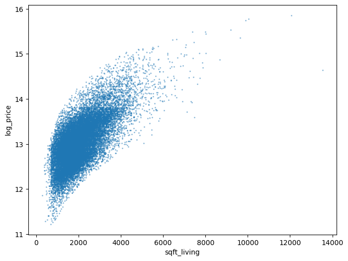
Here’s what the log house price looks like against sqft_living:

def var_scatter(df, ax=None, var="sqft_living"):
    if ax is None:
        _, ax = plt.subplots(figsize=(8, 6))
    df.plot.scatter(x=var , y="log_price", alpha=0.35, s=1.5, ax=ax)

    return ax

var_scatter(df);

Linear Regression

Let’s dive in by studying the “Hello World” of regression algorithms: linear regression.

Suppose we would like to predict the log of the sale price of a home, given only the livable square footage of the home.

The linear regression model for this situation is

\[ \log(\text{price}) = \beta_0 + \beta_1 \text{sqft_living} + \epsilon \]

\( \beta_0 \) and \( \beta_1 \) are called parameters (also coefficients or weights). The machine learning algorithm is tasked with finding the parameter values that best fit the data.

\( \epsilon \) is the error term. It would be unusual for the observed \( \log(\text{price}) \) to be an exact linear function of \( \text{sqft_living} \). The error term captures the deviation of \( \log(\text{price}) \) from a linear function of \( \text{sqft_living} \).

The linear regression algorithm will choose the parameters that minimize the mean squared error (MSE) function, which for our example is written.

\[ \frac{1}{N} \sum_{i=1}^N \left(\log(\text{price}_i) - (\beta_0 + \beta_1 \text{sqft_living}_i) \right)^2 \]

The output of this algorithm is the straight line (hence linear) that passes as close to the points on our scatter chart as possible.

The sns.lmplot function below will plot our scatter chart and draw the optimal linear regression line through the data.

sns.lmplot(
    data=df, x="sqft_living", y="log_price", height=6,
    scatter_kws=dict(s=1.5, alpha=0.35)
);

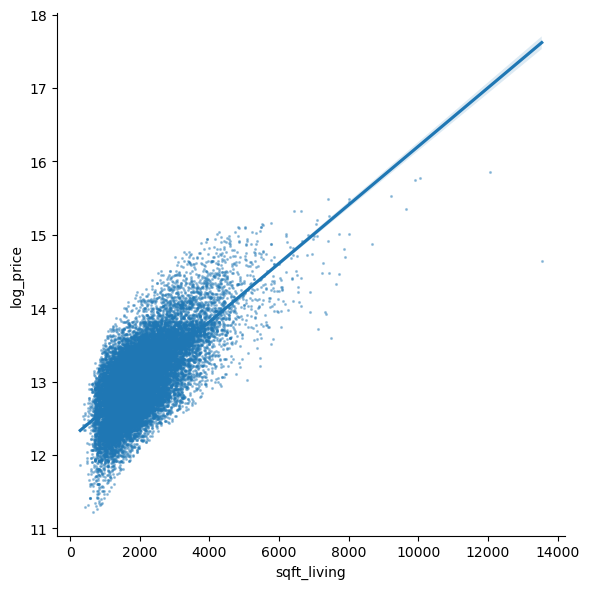
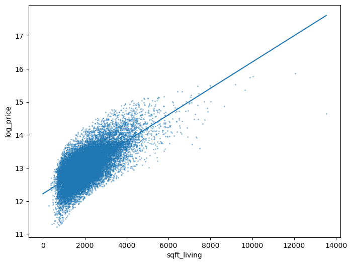
Let’s use sklearn to replicate the figure ourselves.

First, we fit the model.

# import
from sklearn import linear_model

# construct the model instance
sqft_lr_model = linear_model.LinearRegression()

# fit the model
sqft_lr_model.fit(X[["sqft_living"]], y)

# print the coefficients
beta_0 = sqft_lr_model.intercept_
beta_1 = sqft_lr_model.coef_[0]

print(f"Fit model: log(price) = {beta_0:.4f} + {beta_1:.4f} sqft_living")

Fit model: log(price) = 12.2185 + 0.0004 sqft_living

Then, we construct the plot.

ax = var_scatter(df)

# points for the line
x = np.array([0, df["sqft_living"].max()])
ax.plot(x, beta_0 + beta_1*x)

[<matplotlib.lines.Line2D at 0x150bcf1a0d0>]

We can call the predict method on our model to evaluate the model at arbitrary points.

For example, we can ask the model to predict the sale price of a 5,000-square-foot home.

# Note, the argument needs to be two-dimensional. You'll see why shortly.
logp_5000 = sqft_lr_model.predict([[5000]])[0]
print(f"The model predicts a 5,000 sq. foot home would cost {np.exp(logp_5000):.2f} dollars")

The model predicts a 5,000 sq. foot home would cost 1486889.32 dollars

c:\Users\Miguel\anaconda3\envs\econ5129_labs\Lib\site-packages\sklearn\base.py:439: UserWarning: X does not have valid feature names, but LinearRegression was fitted with feature names
  warnings.warn(

Exercise 1

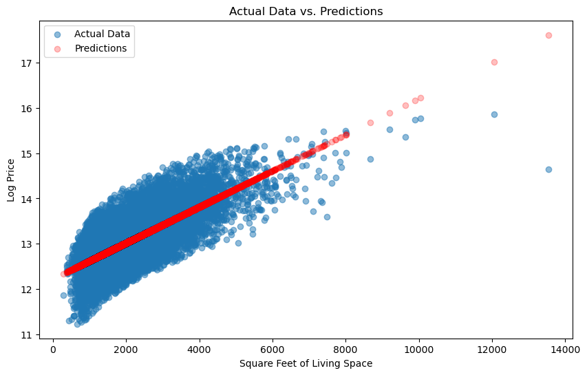
Use the sqft_lr_model that we fit to generate predictions for all data points in our sample.

Note that you need to pass a DataFrame (not Series) containing the sqft_living column to the predict. (See how we passed that to .fit above for help)

Make a scatter chart with the actual data and the predictions on the same figure. Does it look familiar?

When making the scatter for model predictions, we recommend passing c="red" and alpha=0.25 so you can distinguish the data from predictions.

# your code goes here

Solution:

# Generate predictions for all data points
predictions = sqft_lr_model.predict(X[["sqft_living"]])

# Create a scatter plot
plt.figure(figsize=(10, 6))
plt.scatter(X["sqft_living"], y, label="Actual Data", alpha=0.5)
plt.scatter(X["sqft_living"], predictions, c="red", alpha=0.25, label="Predictions")
plt.xlabel("Square Feet of Living Space")
plt.ylabel("Log Price")
plt.legend()
plt.title("Actual Data vs. Predictions")
plt.show()

Exercise 2

Use the metrics.mean_squared_error function to evaluate the loss function used by sklearn when it fits the model for us.

Read the docstring to learn which the arguments that function takes.

from sklearn import metrics

Solutions:

from sklearn.metrics import mean_squared_error

# Calculate mean squared error
mse = mean_squared_error(y, predictions)

print(f"Mean Squared Error: {mse:.2f}")

Mean Squared Error: 0.14

Multivariate Linear Regression

Our example regression above is called a univariate linear regression since it uses a single feature.

In practice, more features would be used.

Suppose that in addition to sqft_living, we also wanted to use the bathrooms variable.

In this case, the linear regression model is

\[ \log(\text{price}) = \beta_0 + \beta_1 \text{sqft_living} + \beta_2 \text{bathrooms} + \epsilon \]

We could keep adding one variable at a time, along with a new \( \beta_{j} \) coefficient for the :math:jth variable, but there’s an easier way.

Let’s write this equation in vector/matrix form as

\[\begin{split} \underbrace{\begin{bmatrix} \log(\text{price}_1) \\ \log(\text{price}_2) \\ \vdots \\ \log(\text{price}_N)\end{bmatrix}}_Y = \underbrace{\begin{bmatrix} 1 & \text{sqft_living}_1 & \text{bathrooms}_1 \\ 1 & \text{sqft_living}_2 & \text{bathrooms}_2 \\ \vdots & \vdots & \vdots \\ 1 & \text{sqft_living}_N & \text{bathrooms}_N \end{bmatrix}}_{X} \underbrace{\begin{bmatrix} \beta_0 \\ \beta_1 \\ \beta_2 \end{bmatrix}}_{\beta} + \epsilon \end{split}\]

Notice that we can add as many columns to \( X \) as we’d like and the linear regression model will still be written \( Y = X \beta + \epsilon \).

The mean squared error loss function for the general model is

\[ \frac{1}{N} \sum_{i=1}^N (y_i - X_i \beta)^2 = \frac{1}{N} \| y - X \beta\|_2^2 \]

where \( || \cdot ||_2 \) is the l2-norm.

Let’s fit the linear regression model using all columns in X.

lr_model = linear_model.LinearRegression()
lr_model.fit(X, y)

LinearRegression()

In a Jupyter environment, please rerun this cell to show the HTML representation or trust the notebook.
On GitHub, the HTML representation is unable to render, please try loading this page with nbviewer.org.

We just fit a model with 18 variables – just as quickly and easily as fitting the model with 1 variable!

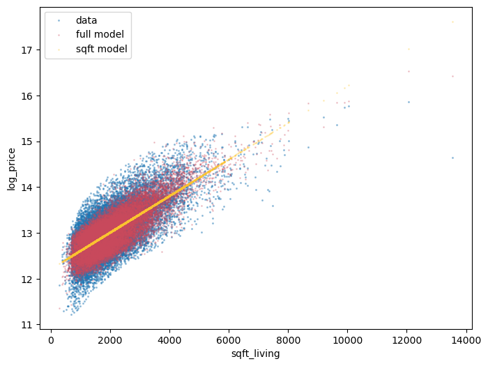
Visualizing a 18-dimensional model is rather difficult, but just so we can see how the extra features changed our model, let’s make the log price vs sqft_living one more time – this time including the prediction from both of our linear models.

ax = var_scatter(df)

def scatter_model(mod, X, ax=None, color=colors[1], x="sqft_living"):
    if ax is None:
        _, ax = plt.subplots()

    ax.scatter(X[x], mod.predict(X), c=color, alpha=0.25, s=1)
    return ax

scatter_model(lr_model, X, ax, color=colors[1])
scatter_model(sqft_lr_model, X[["sqft_living"]], ax, color=colors[2])
ax.legend(["data", "full model", "sqft model"])

<matplotlib.legend.Legend at 0x150bd190bd0>

Exercise 3

Compare the mean squared error for the lr_model and the sqft_lr_model.

Which model has a better fit? Defend your choice.

Solutions:

from sklearn.metrics import mean_squared_error

# Calculate MSE for lr_model
predictions_lr = lr_model.predict(X)
mse_lr = mean_squared_error(y, predictions_lr)

# Calculate MSE for sqft_lr_model
predictions_sqft_lr = sqft_lr_model.predict(X[["sqft_living"]])
mse_sqft_lr = mean_squared_error(y, predictions_sqft_lr)

print(f"Mean Squared Error for lr_model: {mse_lr:.2f}")
print(f"Mean Squared Error for sqft_lr_model: {mse_sqft_lr:.2f}")

Mean Squared Error for lr_model: 0.06
Mean Squared Error for sqft_lr_model: 0.14

Nonlinear Relationships in Linear Regression

While it sounds like an oxymoron, a linear regression model can actually include non-linear features.

The distinguishing feature of the linear regression model is that each prediction is generated by taking the dot product (a linear operator) between a feature vector (one row of \( X \)) and a coefficient vector (\( \beta \)).

There is, however, no restriction on what element we include in our feature vector.

Let’s consider an example…

Starting from the sqft_living-only model, suppose we have a hunch that we should also include the fraction of square feet above ground.

This last variable can be computed as sqft_above / sqft_living.

This second feature is nonlinear, but could easily be included as a column in X.

Let’s see this in action.

X2 = X[["sqft_living"]].copy()
X2["pct_sqft_above"] = X["sqft_above"] / X["sqft_living"]

sqft_above_lr_model = linear_model.LinearRegression()
sqft_above_lr_model.fit(X2, y)

new_mse = metrics.mean_squared_error(y, sqft_above_lr_model.predict(X2))
old_mse = metrics.mean_squared_error(y, sqft_lr_model.predict(X2[["sqft_living"]]))
print(f"The mse changed from {old_mse:.4f} to {new_mse:.4f} by including our new feature")

The mse changed from 0.1433 to 0.1430 by including our new feature

Exercise 4

Explore how you can improve the fit of the full model by adding additional features created from the existing ones.

# your code here

Solutions:

In this example, we created polynomial features of degree 2 from the existing features and fitted a linear regression model with these polynomial features. You can adapt this code to include other feature engineering techniques and evaluate their impact on model fit. Remember to use proper evaluation metrics and cross-validation to assess the model’s performance effectively.

from sklearn.preprocessing import PolynomialFeatures

# Create polynomial features
poly = PolynomialFeatures(degree=2)
X_poly = poly.fit_transform(X)

# Fit a new model with polynomial features
lr_poly_model = linear_model.LinearRegression()
lr_poly_model.fit(X_poly, y)

# Calculate MSE for the model with polynomial features
predictions_poly = lr_poly_model.predict(X_poly)
mse_poly = mean_squared_error(y, predictions_poly)

print(f"Mean Squared Error for lr_poly_model: {mse_poly:.2f}")

Mean Squared Error for lr_poly_model: 0.05

Determining which columns belong in \( X \) is called feature engineering and is a large part of a machine learning practitioner’s job.

You may recall from (or will see in) your econometrics course(s) that choosing which control variables to include in a regression model is an important part of applied research.

Interpretability

Before moving to our next regression model, we want to broach the idea of the interpretability of models.

An interpretable model is one for which we can analyze the coefficients to explain why it makes its predictions.

Recall \( \beta_0 \) and \( \beta_1 \) from the univariate model.

The interpretation of the model is that \( \beta_0 \) captures the notion of the average or starting house price and \( \beta_1 \) is the additional value per square foot.

Concretely, we have

beta_0, beta_1

(12.218464096380853, 0.0003987465387451502)

which means that our model predicts the log price of a house to be 12.22, plus an additional 0.0004 for every square foot.

Using more exotic machine learning methods might potentially be more accurate but less interpretable.

The accuracy vs interpretability tradeoff is a hot discussion topic, especially relating to concepts like machine learning ethics. This is something you should be aware of as you continue to learn about these techniques.

References

Some good text books covering the above regression methods:

Christopher M. Bishop. Pattern Recognition and Machine Learning. Springer, 2006.

Bradley Efron and Trevor Hastie. Computer age statistical inference. Volume 5. Cambridge University Press, 2016.

Jerome Friedman, Trevor Hastie, and Robert Tibshirani. The elements of statistical learning. Springer series in statistics, 2009..