
Logistic Regression#
We will spend the entire lab today building simple models that predicts recessions. Let’s follow Favara et al, 2016 and model
Where \(NBER_t\) is a dummy variable equal to 1 if the economy is in recession in month t and 0 otherwise. \(X\) denotes the features matrix and includes a constant, \(S_t^{GZ}\) a measure of credit spreads, \(EBP_t\) the excess loan premium that measures credit spreads that are orthogonal to defaults, \(TS_t\) is the term-spread and the \(TBill_t\) is the 3 month T-bill yield. Instead of using a probit model, let’s instead use a logistic regression to explore the problem of predicting a recession.
Next, we will extend this simple model in the lines of Vrontos, Galakis and Vrontos, 2021, augmenting it with 134 variables available in the FRED-MD database and use appropriate regularization to tame parameter proliferation.
Start by loading the materials of the Federal Reserve Bank of New York’s ‘The Yield Curve as a Leading Indicator’ and FRED. Then, consider alternative models in and augment the space of predictors.
#!pip install pandas-datareader
#!pip install xlrd
import warnings
import requests
from skimpy import skim
import pandas as pd
import pandas_datareader as pdr
import datetime
# Turn off warnings
warnings.filterwarnings("ignore")

# Download the data from the various sources
url_1 = "https://www.newyorkfed.org/medialibrary/media/research/capital_markets/allmonth.xls"
url_2= "https://www.federalreserve.gov/econresdata/notes/feds-notes/2016/files/ebp_csv.csv"

# get the data for NBER, TS, TBill
getit = requests.get(url_1)
with open("data_nyfed.xls", "wb") as f:
    f.write(getit.content)
# load the data to working environemnt
df1 = pd.read_excel("data_nyfed.xls")

# get the data for GZ spread and EBP
getit_ = requests.get(url_2)
with open("data_ebp.csv", "wb",) as f:
    f.write(getit_.content)
df2 = pd.read_csv("data_ebp.csv")

# get the FRED-MD data (download it from Moodle and load)
# Note that I already pre-processed the data to ensure stationarity
df3 = pd.read_csv("fred_md.csv")

# Merge the DataFrames using 'date' as the common column
df1['Date'] = pd.to_datetime(df1['Date'] )
df2['date'] = pd.to_datetime(df2['date'] )
df3['date'] = pd.to_datetime(df2['date'] )

# Extract month and year from 'Date' columns and create a new column 'MonthYear'
df1['MonthYear'] = df1['Date'].dt.strftime('%Y-%m')
df2['MonthYear'] = df2['date'].dt.strftime('%Y-%m')
df3['MonthYear'] = df3['date'].dt.strftime('%Y-%m')

# merge them all in a single DataFrame
data_all = pd.merge(df1, df2, on='MonthYear', how='inner').merge(df3, on='MonthYear', how='inner')

skim(data_all)
---------------------------------------------------------------------------
ModuleNotFoundError                       Traceback (most recent call last)
Cell In[1], line 5
      3 import warnings
      4 import requests
----> 5 from skimpy import skim
      6 import pandas as pd
      7 import pandas_datareader as pdr

ModuleNotFoundError: No module named 'skimpy'
Our variable of interest is NBER_Rec that equals 1 for time-periods in a recession and 0 otherwise. As predictors we’ll use:
The 3 Month Treasury Yield ,
The 10Y-3M term-spread,
The GZ Spread
The Excess Bond Premium (EBP)
Let’s plot some descriptives of the term-spread and the NBER Recession dummy.
import matplotlib.pyplot as plt

# Create a plot with two y-axes
fig, ax1 = plt.subplots()

# Plot the first time series on the left y-axis
ax1.plot(data_all['Date'], data_all['Spread'], color='b')
ax1.set_xlabel('Date')
ax1.set_ylabel('Spread', color='b')
ax1.tick_params('y', colors='b')

# Create a second y-axis on the right side for the dummy variable
ax2 = ax1.twinx()
ax2.plot(data_all['Date'], data_all['NBER_Rec'], color='r')
ax2.set_ylabel('NBER_Rec', color='r')
ax2.tick_params('y', colors='r')

# Set the title and display the plot
plt.title('Time Series of {} and {}'.format('Spread', 'NBER_Rec'))
plt.show()
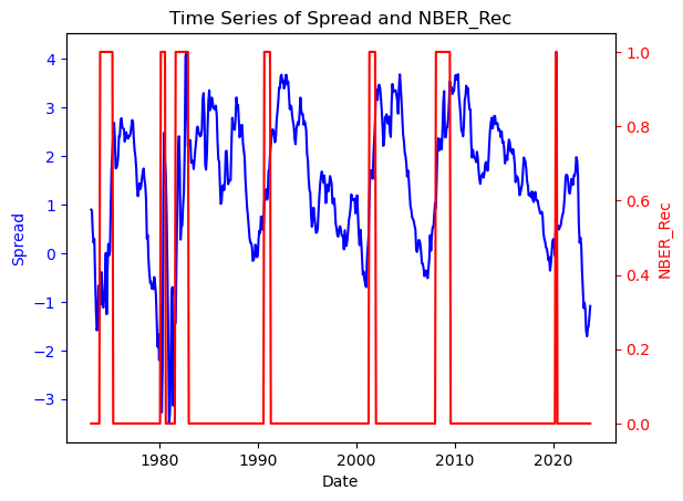
There seems to be a link between Term-spread and Recessions. Notice that before every recession in the past couple of decades in the US, the term spread tends to invert. Let’s look into this more deeply and build a recession preditive model based on the term-spread.
Logistic Regression for Classification#
Objective: Logistic regression is a widely used statistical method for classification tasks in machine learning. It models the probability of a binary outcome as a function of predictor variables, making it well-suited for recession prediction.
Key Points:
Sigmoid Function: Logistic regression uses the sigmoid function \(\sigma(.)\) to transform the output of a linear combination of input features into a value between 0 and 1. The sigmoid function is defined as:
\[P(Y=1|X) = \sigma(Xw)\]
where \(\sigma(a) = 1/(1+exp(-a))\).
Let’s try and fit this model to the data by using the term-spread as a single predictor.
First, create a new variable equal to 1 if a recession occurs between \(\{t,t+12\}\) in months.
import pandas as pd

# Define a function to check if a recession occurs within 12 months ahead
def recession_in_next_12_months(row, data):
    current_date = row['Date']
    end_date = current_date + pd.DateOffset(months=12)

    # Filter data for the next 12 months
    next_12_months = data[(data['Date'] > current_date) & (data['Date'] <= end_date)]

    # Check if any of those months had a recession
    if next_12_months['NBER_Rec'].sum() > 0:
        return 1
    else:
        return 0

# Create a new column 'Recession_in_12_Months' using the defined function
data_all['NBER_Rec12'] = data_all.apply(lambda row: recession_in_next_12_months(row, data_all), axis=1)
Now let’s estimate a logistic version of the Probit model in Favara et al, 2016
from sklearn.linear_model import LogisticRegression
from sklearn.metrics import accuracy_score, classification_report
from sklearn.model_selection import train_test_split

# Define the independent variable (Term_Spread) and the dependent variable (Recession_Label)
X = data_all[['TB3MS','Spread','gz_spread','ebp']]
y = data_all[['NBER_Rec12']]
X = (X-X.mean())/X.std()
# Fill missing values with zeros
X.fillna(0, inplace=True)
# Define the cutoff date for splitting
cutoff_date = '2010-01-01'

# Use the cutoff date to separate the training and testing sets
X_train = X[data_all['Date'] < cutoff_date]
y_train = y[data_all['Date'] < cutoff_date]
X_test= X[data_all['Date'] >= cutoff_date]
y_test = y[data_all['Date'] >= cutoff_date]

# Create and fit a logistic regression model
model = LogisticRegression()
model.fit(X_train, y_train)

# Make predictions on the test set
y_pred = model.predict(X_test)

# Calculate and print accuracy
accuracy = accuracy_score(y_test, y_pred)
print(f"Accuracy: {accuracy:.2f}")

# Print a classification report with additional metrics
report = classification_report(y_test, y_pred)
print("Classification Report:\n", report)

# Now, let's use the trained model to predict a recession probability for a new data point
recession_probability = model.predict_proba(X)
data_all['rp'] = recession_probability[:,1]
Accuracy: 0.85
Classification Report:
               precision    recall  f1-score   support

           0       0.95      0.88      0.91       152
           1       0.25      0.46      0.32        13

    accuracy                           0.85       165
   macro avg       0.60      0.67      0.62       165
weighted avg       0.90      0.85      0.87       165
Let’s have a look at our recession probability indicator
import matplotlib.pyplot as plt

# Create a figure with two subplots side by side
fig, (ax1, ax2) = plt.subplots(1, 2, figsize=(16, 6))

# Plot the first time series on the left subplot
ax1.plot(data_all['Date'], data_all['rp'], color='b')
ax1.set_xlabel('Date')
ax1.set_ylabel('Recession Prob.', color='b')
ax1.tick_params('y', colors='b')

# Create a second y-axis on the right side for the dummy variable on the left subplot
ax2_1 = ax1.twinx()
ax2_1.plot(data_all['Date'], data_all['NBER_Rec'], color='r')
ax2_1.set_ylabel('NBER_Rec', color='r')
ax2_1.tick_params('y', colors='r')

# Plot the second time series on the right subplot
ax2.plot(data_all['Date'], data_all['est_prob'], color='g')  # Replace 'Another_Variable' with your column name
ax2.set_xlabel('Date')
ax2.set_ylabel('Recession Prob.', color='g')
ax2.tick_params('y', colors='g')

# Set the titles for both subplots
ax1.set_title('Time Series of {} and {}'.format('Logit Recession Prob.', 'NBER_Rec'))
ax2.set_title('Time Series of {} {}'.format('Recession Prob. as calculated by the NYFED', ''))

# Adjust the layout for better spacing
plt.tight_layout()

# Display the plot
plt.show()
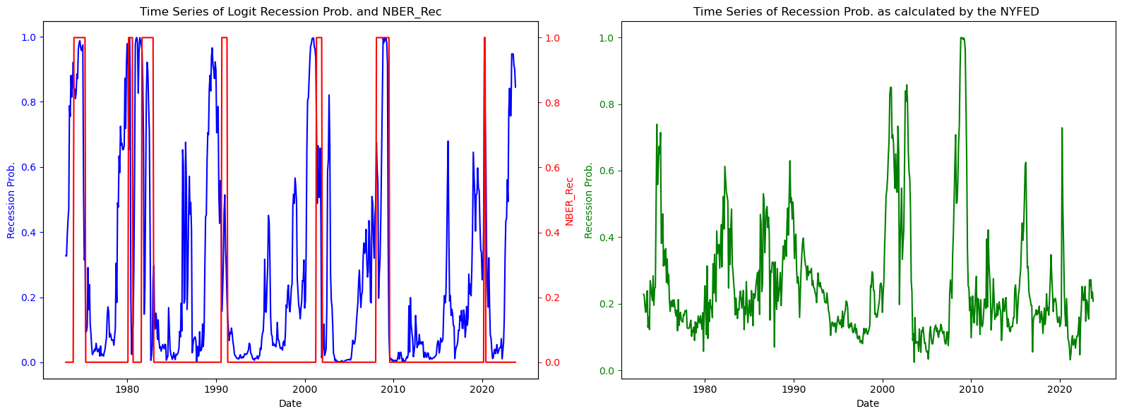
The green line on the right panel in the figure above plots the New York Feds Probability of Recession indicator.
Which one performs better ? To compare our Logistic models with the Probit, let’s estimate a probit and look at model evaluation statistics.
from statsmodels.discrete.discrete_model import Probit
from sklearn.linear_model import LogisticRegression

# Logistic regression model
logit_model = LogisticRegression()
logit_model.fit(X_train, y_train)

# Probit regression model
probit_model = Probit(y_train, X_train)
probit_result = probit_model.fit()

# Logistic regression predictions
logit_predictions = logit_model.predict(X_test)
logit_accuracy = accuracy_score(y_test, logit_predictions)
print("Logistic Regression Accuracy:", logit_accuracy)
print(classification_report(y_test, logit_predictions))

# Probit regression predictions
probit_predictions = probit_result.predict(X_test)
probit_predictions = (probit_predictions > 0.5).astype(int)
probit_accuracy = accuracy_score(y_test, probit_predictions)
print("Probit Regression Accuracy:", probit_accuracy)
print(classification_report(y_test, probit_predictions))


logit_probabilities = logit_model.predict_proba(X)[:, 1]
probit_probabilities = probit_result.predict(X)
# Now, let's use the trained model to predict a recession probability for a new data point

data_all['rp_probit'] = probit_probabilities
data_all['rp_logistic'] = logit_probabilities
Optimization terminated successfully.
         Current function value: 0.457587
         Iterations 6
Logistic Regression Accuracy: 0.8484848484848485
              precision    recall  f1-score   support

           0       0.95      0.88      0.91       152
           1       0.25      0.46      0.32        13

    accuracy                           0.85       165
   macro avg       0.60      0.67      0.62       165
weighted avg       0.90      0.85      0.87       165

Probit Regression Accuracy: 0.703030303030303
              precision    recall  f1-score   support

           0       1.00      0.68      0.81       152
           1       0.21      1.00      0.35        13

    accuracy                           0.70       165
   macro avg       0.60      0.84      0.58       165
weighted avg       0.94      0.70      0.77       165
# Create a figure
fig, ax = plt.subplots(figsize=(11, 3))

# Plot the Probit recession probability in blue
ax.plot(data_all['Date'], data_all['rp_probit'], color='b', label='Recession Probability (Probit)')
ax.plot(data_all['Date'], data_all['rp_logistic'], color='k', linestyle='dotted', label='Recession Probability (Logistic)')

# Set the x/y-axis label
ax.set_xlabel('Date')
ax.set_ylabel('Recession Probability', color='k')
plt.tight_layout()

# Display a legend
ax.legend(loc='upper left')
plt.show()
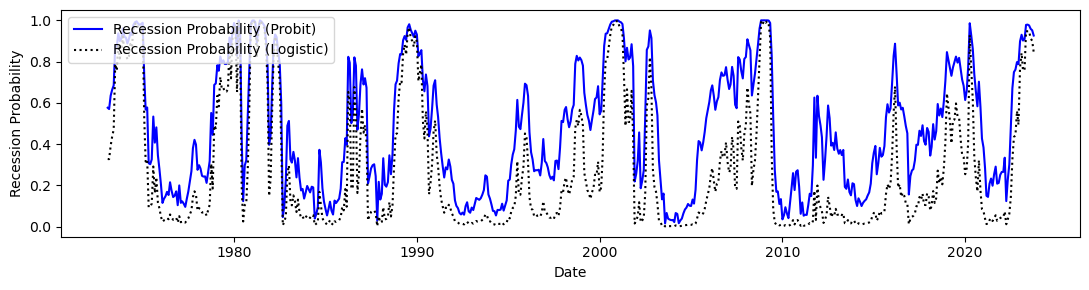
Our model seems to slightly outperform the NYFED. Let’s now enlarge the information set by considering the 134 variables in FRED-MD and use appropriate regularization methods as learnt in previous lectures & labs.
from sklearn.linear_model import LogisticRegression
from sklearn.metrics import accuracy_score, classification_report
from sklearn.model_selection import train_test_split

# Define the independent variable (Term_Spread) and the dependent variable (Recession_Label)
X = data_all.drop(['Date','MonthYear','NBER_Rec','NBER_Rec12','Rec_prob','date_x','date_y','est_prob','est_prob','NBER_Rec12','rp_probit','rp_logistic','rp'], axis=1)
y = data_all[['NBER_Rec12']]
X = (X-X.mean())/X.std()
# Fill missing values with zeros
X.fillna(0, inplace=True)
# Define the cutoff date for splitting
cutoff_date = '2010-01-01'

# Use the cutoff date to separate the training and testing sets
X_train = X[data_all['Date'] < cutoff_date]
y_train = y[data_all['Date'] < cutoff_date]
X_test= X[data_all['Date'] >= cutoff_date]
y_test = y[data_all['Date'] >= cutoff_date]

# Create and fit a logistic regression model with L1 (Lasso) regularization
# You can adjust the 'C' parameter to control the strength of regularization.
# Smaller 'C' values add more regularization.
model = LogisticRegression(penalty='l1', C=1.0, solver='liblinear')  # Adjust C as needed; penalty='l2' => Ridge
model.fit(X_train, y_train)

# Make predictions on the test set
y_pred = model.predict(X_test)

# Calculate and print accuracy
accuracy = accuracy_score(y_test, y_pred)
print(f"Accuracy: {accuracy:.2f}")

# Print a classification report with additional metrics
report = classification_report(y_test, y_pred)
print("Classification Report:\n", report)

# Now, let's use the trained model to predict a recession probability for a new data point
recession_probability = model.predict_proba(X)
data_all['rp'] = recession_probability[:,1]
Accuracy: 0.88
Classification Report:
               precision    recall  f1-score   support

           0       0.92      0.96      0.94       152
           1       0.00      0.00      0.00        13

    accuracy                           0.88       165
   macro avg       0.46      0.48      0.47       165
weighted avg       0.85      0.88      0.86       165
Gains in terms of accuracy are modest but this model seems to be best. It may be of interest to examine which variables are chosen by Lasso as predictors of recessions:
# Get the coefficients (weights) of the model after L1 regularization
coef = model.coef_[0]
variable_names = X.columns
# Print the coefficients and corresponding variable names
print("Coefficients for each variable:")
i = 0
for name, weight in zip(variable_names, coef):
    if weight != 0:  # Only print variables with non-zero coefficients
        print(f"{name}: {weight:.4f}")
        i += 1

print('The model selects ' + str(i) + ' variables out of a total of ' + str(X.shape[1]))
Coefficients for each variable:
3 Month Treasury Yield: 0.7199
3 Month Treasury Yield (Bond Equivalent Basis): 1.2656
Spread: -1.2969
gz_spread: 0.7133
ebp: 1.5605
RPI: 0.1059
DPCERA3M086SBEA: -0.2118
IPDCONGD: -0.3112
IPBUSEQ: 0.2764
IPDMAT: -0.1923
IPNMAT: 0.0249
IPB51222S: 0.1769
IPFUELS: 0.1316
HWI: 0.1817
UNRATE: 0.1088
UEMPMEAN: -0.0520
UEMPLT5: -0.2557
UEMP5TO14: -0.0146
UEMP15T26: -0.1380
UEMP27OV: 0.0118
CES1021000001: 0.0640
DMANEMP: 0.2930
NDMANEMP: -0.1358
SRVPRD: -0.2063
USTRADE: 0.0266
USFIRE: 1.1891
AWOTMAN: -0.1337
AWHMAN: 1.7073
HOUSTMW: 0.5146
HOUSTS: -1.6924
HOUSTW: 0.4511
PERMITNE: -1.0099
PERMITMW: 0.5022
AMDMNOx: -0.2554
ANDENOx: 0.2160
M2REAL: 0.3988
BOGMBASE: 0.0175
TOTRESNS: 0.0991
REALLN: 0.1642
NONREVSL: -0.1435
CONSPI: 0.4921
S&P 500: 0.2635
S&P PE ratio: -0.0267
CP3Mx: -0.2420
TB3MS: -0.0820
TB6MS: -0.0094
GS1: -0.2227
BAA: 0.4518
COMPAPFFx: 0.5345
T1YFFM: 0.7425
AAAFFM: 0.3067
TWEXAFEGSMTHx: -0.1384
EXUSUKx: 0.2891
WPSFD49207: -0.1449
WPSID61: -0.1029
OILPRICEx: -0.2997
CPIAUCSL: 0.2194
CPITRNSL: -0.0020
CPIMEDSL: -0.1677
CPIULFSL: -0.1096
DSERRG3M086SBEA: 0.0656
CES0600000008: 0.0761
CES3000000008: 0.0377
DTCTHFNM: 0.1676
INVEST: 0.1599
VIXCLSx: 0.1415
mu_3: -1.2070
fi_1: 0.1462
fi_12: 0.6688
The model selects 69 variables out of a total of 140
Exercise#
Change the regularization scheme and comment on how the results change.
References#
Federal Reserve Bank of New York, The Yield Curve as a Leading Indicator.
Vrontos, Spyridon D. & Galakis, John & Vrontos, Ioannis D., 2021. “Modeling and predicting U.S. recessions using machine learning techniques,” International Journal of Forecasting, Elsevier, vol. 37(2), pages 647-671.
Favara, Giovanni, Simon Gilchrist, Kurt F. Lewis, and Egon Zakrajsek (2016). “Recession Risk and the Excess Bond Premium,” FEDS Notes. Washington: Board of Governors of the Federal Reserve System, April 8, 2016.